TiRank Web App Tutorial

This tutorial provides a complete walkthrough of the TiRank web application.

Note

This documentation references several images (e.g., load-data-tutorial.png). For these images to display correctly when you build the documentation locally, please copy all image files from your project’s Web/assets/ directory into the docs/source/_static/ directory.

Introduction of TiRank Web

The TiRank web application is built with the Python Dash framework (https://dash.plotly.com). TiRank-web is organized into six sections: Homepage, Upload Data, Pre-processing, Analysis, Tutorial, and FAQs.

In Upload Data, users provide datasets that TiRank organizes into designated folders for temporary storage and figure generation. Pre-processing covers data cleaning, normalization, and splitting (training/validation) for hyperparameter optimization, and prepares the binary gene-pair matrix for downstream modeling. The Analysis section trains the model, computes TiRank scores, and supports differential expression and pathway enrichment.

Video Tutorial of TiRank Web

The archived, citable GUI tutorial video is hosted on Zenodo:

• Zenodo DOI: https://doi.org/10.5281/zenodo.18275554

Download the GUI tutorial video (TiRank GUI Tutorial.mp4) from Zenodo.

(Optional) Streaming mirror (non-archival): https://www.youtube.com/watch?v=YMflTzJF6s8

---

1. UploadData

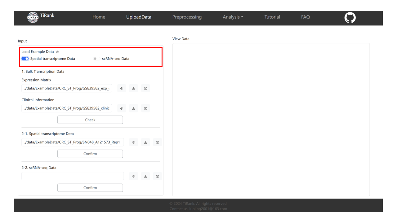
1.1 Load Example Data

We provide exemplary datasets for both Spatial Transcriptomics (ST) and scRNA-seq. The archived example datasets are available from Zenodo (see DOI above). The Zenodo record includes:

• ExampleData.zip (example datasets)

• ctranspath.pth (pretrained model file)

• TiRank GUI Tutorial.mp4 (GUI tutorial video)

To use the “Load Example Data” buttons in the local GUI, ensure the example datasets and pretrained model file are extracted and placed under Web/data/ as described in Installation.

In the GUI (right-side panel), users can select either “Spatial Transcriptomics Data” or “scRNA-seq Data”. Once selected, the relevant form fields will be auto-populated with the sample paths.

Hint: Only fill out one of the ST (2-1) or scRNA-seq (2-2) forms.

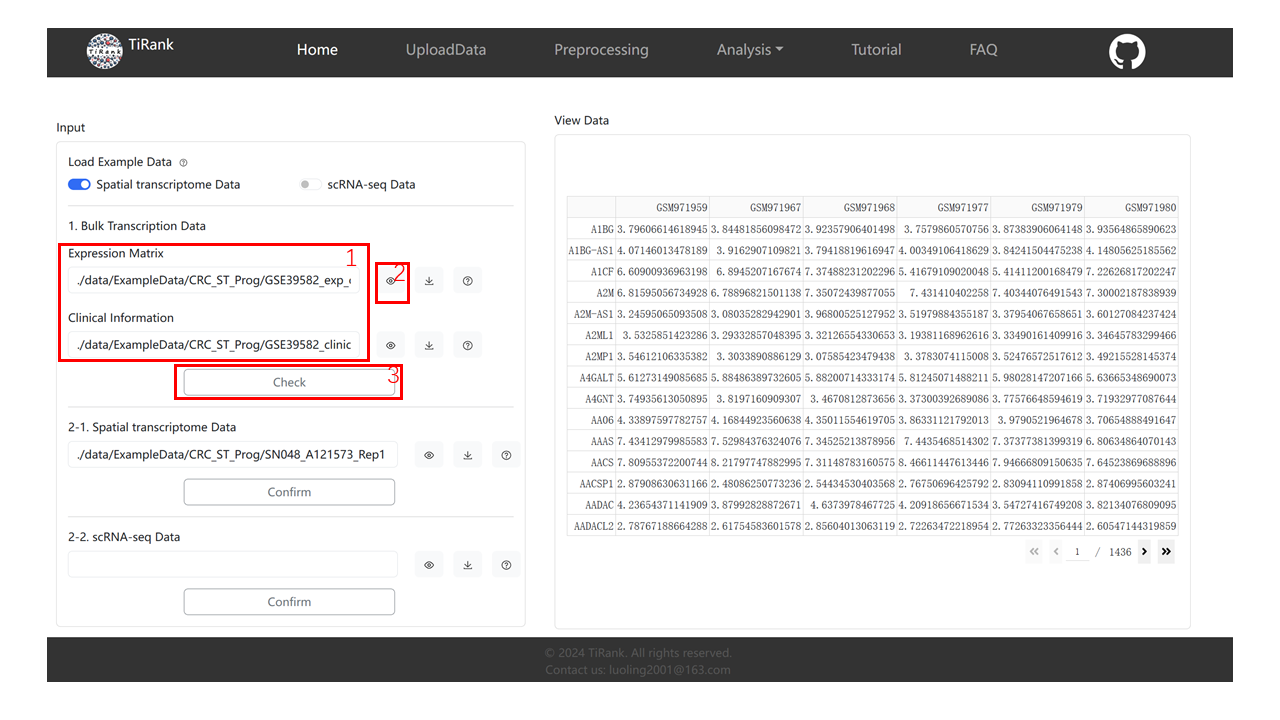
1.2 Bulk Transcription Data

We use the loaded ST example as an illustration.

1. After loading, the paths to the bulk expression matrix and clinical information are automatically filled. You may also enter your own absolute paths manually.

2. Click “View” to visualize the loaded table.

3. Click “Check” to validate input format for TiRank.

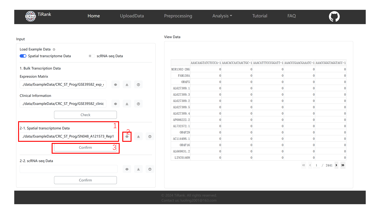
1.3 Spatial transcriptome Data / scRNA-seq Data

1. After loading, the ST (or scRNA-seq) paths are auto-filled; you may also enter your own absolute paths.

2. Click “View” to visualize the loaded data.

3. Click “Confirm” to indicate whether your data is ST or scRNA-seq (required because downstream processing differs).

---

2. Preprocessing

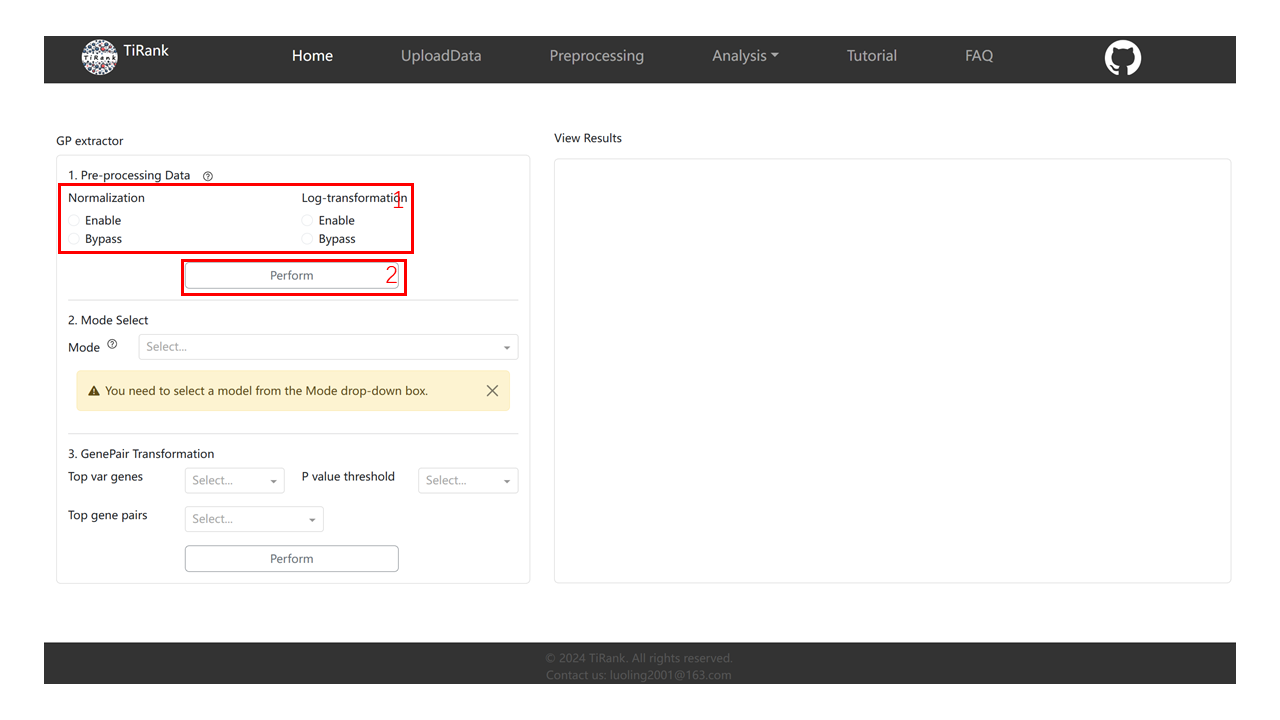
2.1 Pre-processing Data

1. Select “Enable” or “Bypass” for Normalization and Log-transformation.

2. Click “Perform” to preprocess.

Note: The system may show a loading screen for several minutes; please wait until preprocessing completes.

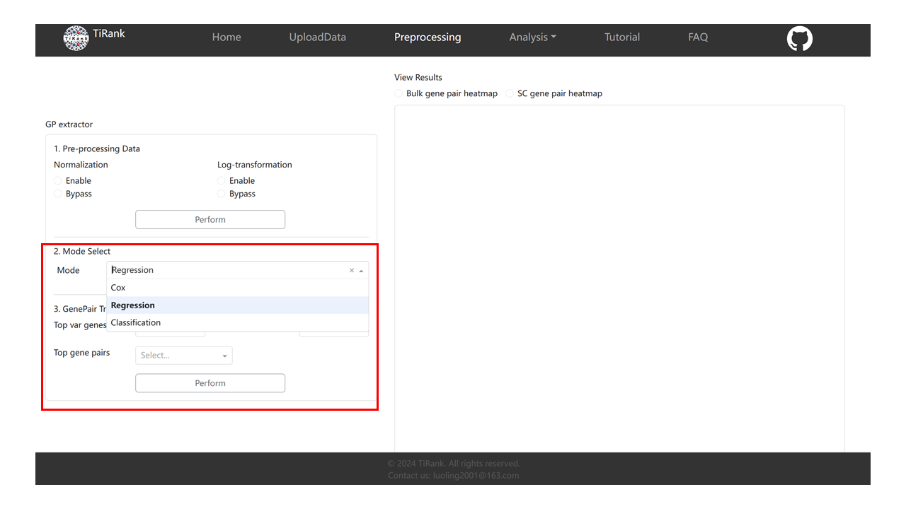
2.2 Mode select And GenePair Transformation

1. Mode select: Choose the mode you want.

2. GenePair Transformation: Select parameters (recommended defaults below), then click “Perform”.

'Top var genes': 2000
'P value threshold': 0.05
'Top gene pairs': 2000

Note: This step may take longer; wait until processing completes.

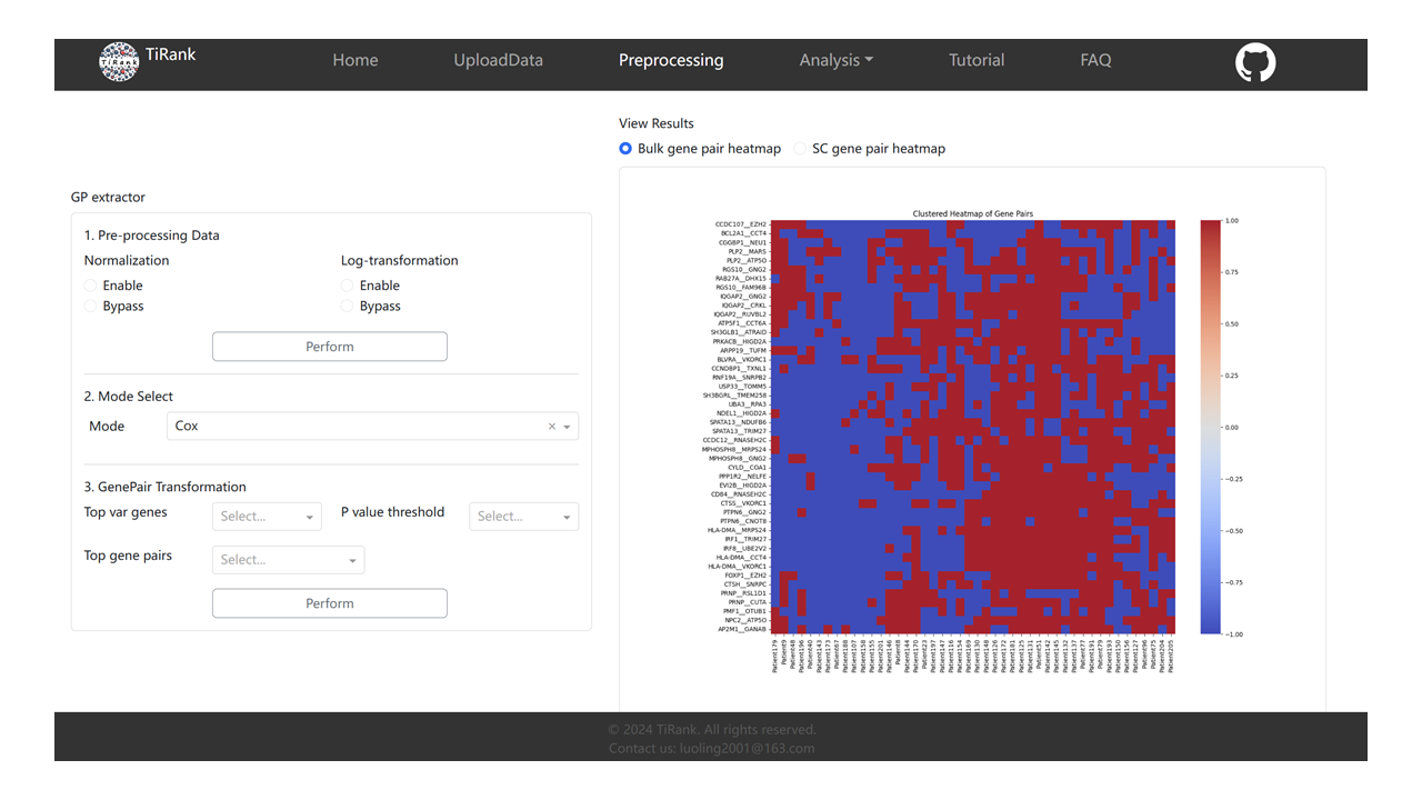
2.3 View Results

After preprocessing and gene-pair transformation, use the radio controls above the right card to select and view result plots.

---

3. Analysis/TiRank

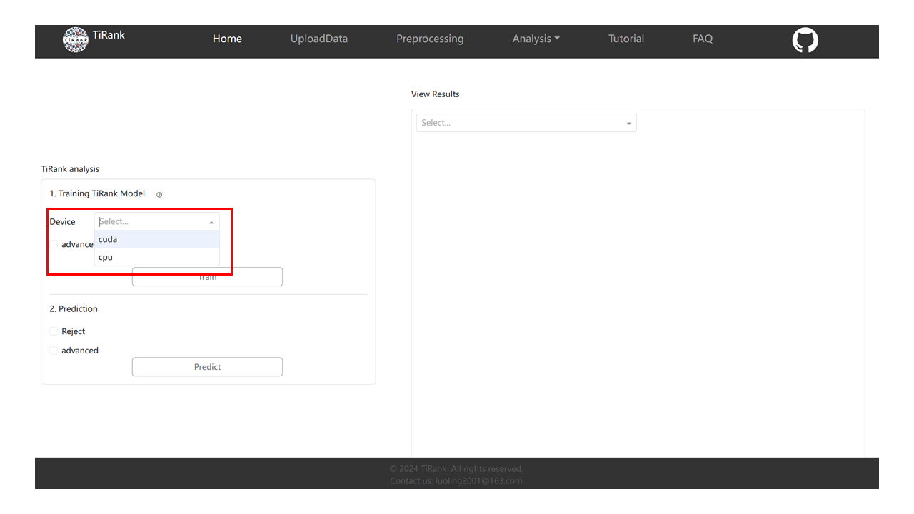
3.1 Device select

Select CPU or GPU. If you use GPU, ensure PyTorch is installed for your CUDA/driver.

Check GPU driver:

nvidia-smi

Check CUDA availability in Python:

import torch
print(torch.cuda.is_available())

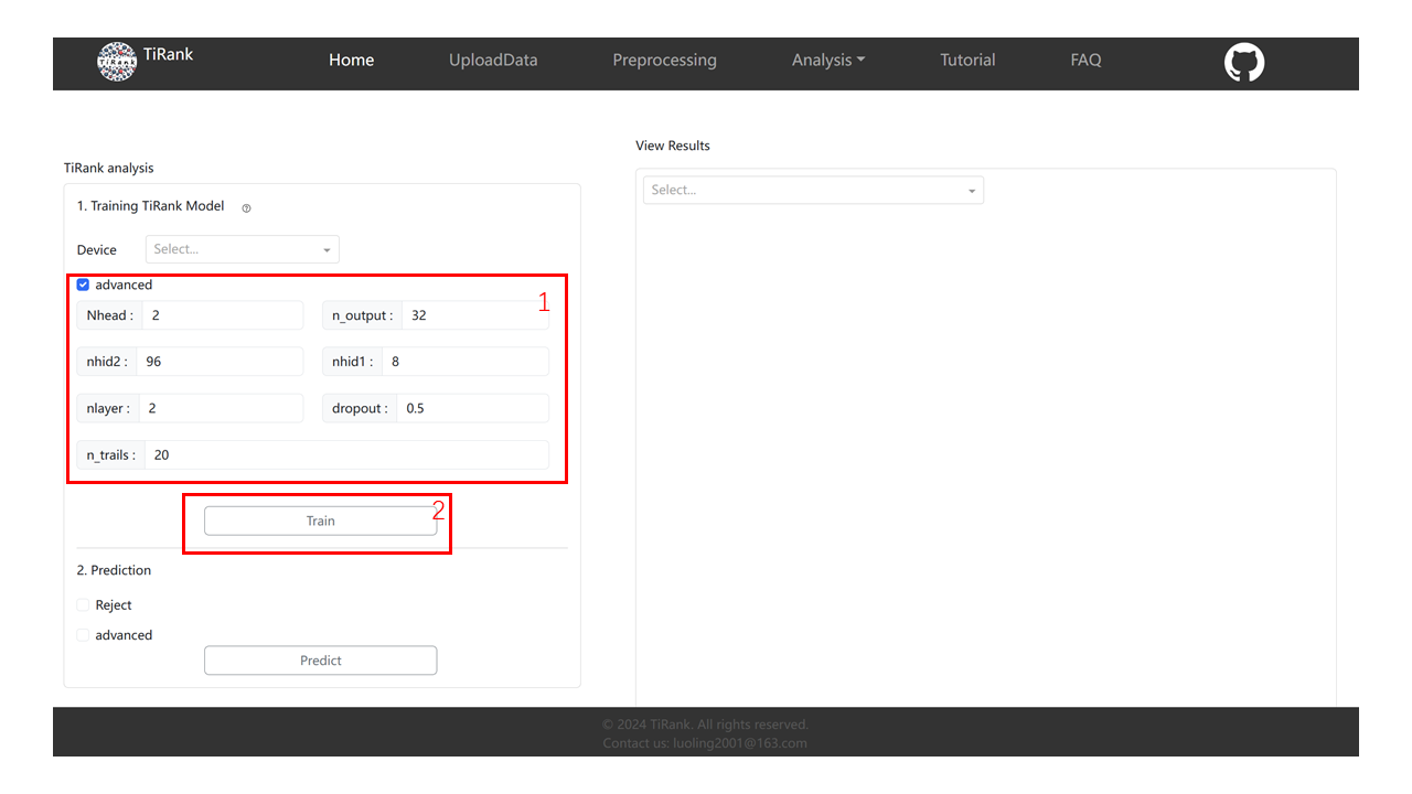
3.2 Training TiRank Model

Optionally click “Advanced” to change parameters. Default parameters:

'Nhead': 2
'n_output': 32
'nhid1': 96
'nhid2': 8
'nlayers': 2
'n_trails': 20
'dropout': 0.5

Click “Train” to start training (this can take time).

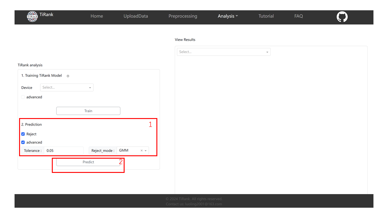
3.3 Prediction

Optionally enable rejection and adjust prediction parameters. Default parameters:

'Tolerance': 0.05
'Reject_mode': 'GMM'

Click “Predict”.

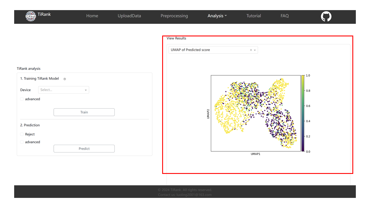
3.4 View Results

After training/prediction, choose result plots from the dropdown menu to view.

---

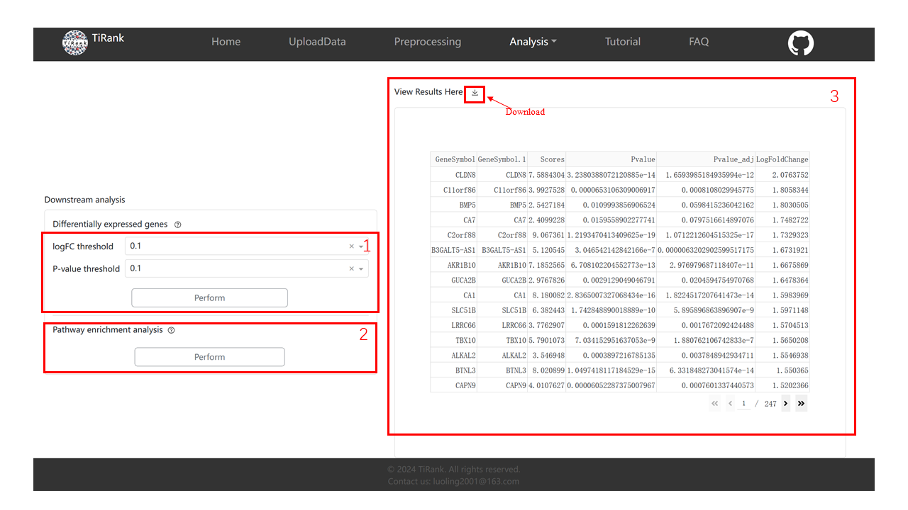
4. Analysis/Differential expression genes & Pathway enrichment

1. Differential expression genes: set logFC and P-value thresholds and click “Perform”.

2. Pathway enrichment: click “Perform”.

3. View Results: inspect results on the right and download if needed.